

The main types of financial forecasting models fall into two broad frameworks, top-down and bottom-up, plus five method families: time-series (moving average, exponential smoothing, ARIMA), regression (simple and multiple), scenario/probabilistic (including Monte Carlo), machine learning/AI, and qualitative methods such as Delphi and expert panels. Choosing among them comes down to three questions: What decision does this forecast serve? How much historical data do you have? And how much explainability do your stakeholders require?
Quick selection rules for the most common situations:
- Short-term cash or sales forecasting (weekly to quarterly): start with exponential smoothing or a simple moving average, then layer in ARIMA if you have at least two years of clean data with detectable seasonality.
- Operational budgeting and pro forma modeling: use a bottom-up driver-based approach — build from units, pricing, and headcount, then validate against a top-down market check.
- Strategic sizing or market-entry planning: top-down with scenario analysis, anchoring macro assumptions to GDP cycles and industry benchmarks from sources like the IMF.
Evaluate every model with MAPE (mean absolute percentage error) and RMSE (root mean squared error) on a held-out test period before trusting it in a live planning cycle. Amcfo's fractional CFO practice uses a hybrid workflow that combines these model families with a structured governance cadence — more on that in the implementation section below.
Key Takeaways
The most reliable financial forecasts combine a bottom-up driver model with a top-down market check, evaluated against MAPE or RMSE on a held-out period, and maintained on a rolling quarterly cadence.
| Point | Details |
|---|---|
| Match model to decision horizon | Short-term cash needs time-series or moving averages; strategic sizing needs top-down with scenario analysis. |
| Validate with hybrid frameworks | Run bottom-up driver forecasts and top-down market checks together; reconcile the gap before presenting to stakeholders. |
| Evaluate on holdout data | Always backtest on data the model never saw; use MAPE for scale-independent comparison and RMSE when large errors are costly. |
| Keep a simple baseline | A moving average or straight-line model running alongside complex models catches model drift and preserves stakeholder trust. |
| Amcfo for implementation | Amcfo builds, integrates, and maintains hybrid forecasting processes for businesses that need reliable forecasts without a full-time CFO. |
Table of Contents
- What are the main types of financial forecasting models?
- Quantitative vs. qualitative: how do these two categories differ?
- Simple methods: percent-of-sales, straight-line, and moving averages
- Time-series methods: exponential smoothing, Holt-Winters, and ARIMA
- How does regression analysis work in financial forecasting?
- Bottom-up vs. top-down: which framework fits your situation?
- Scenario analysis and Monte Carlo: forecasting under uncertainty
- When does machine learning actually improve financial forecasts?
- Qualitative methods: Delphi, expert panels, and market research
- How to choose the right forecasting model for your business
- Inputs, assumptions, and how to evaluate forecast accuracy
- Operationalizing forecasts: cadence, ownership, and common pitfalls
- Amcfo's recommendation: use a hybrid approach with a structured checklist
- What fractional CFOs actually fix in broken forecasting processes
- Amcfo's forecasting and modeling services
- Sources
What are the main types of financial forecasting models?
Financial forecasting is the practice of making informed predictions about future financial outcomes — revenue, expenses, cash flow, or balance sheet positions — using historical data, business drivers, and assumptions about the future. It is not the same as financial modeling, though the two terms get conflated constantly.
IBM draws a clean line between the two: a model is the structured framework that connects your financial statements (income statement, balance sheet, cash flow statement) and defines how inputs flow through to outputs. A method or technique is the mathematical engine inside that model — regression, moving average, ARIMA, and so on. A top-down model can use straight-line growth as its technique. A bottom-up model can use multiple regression. The framework and the technique are separate choices.
Pro forma statements are the output containers. When a forecast is complete, it typically populates a pro forma income statement, a pro forma balance sheet, and a pro forma cash flow statement — the three-statement model that most finance teams use for budgeting, investor presentations, and scenario testing. The forecast feeds the model; the model produces the pro forma.
Where do evaluation metrics fit? MAPE and RMSE are not part of the forecast itself — they measure how well a chosen method performed on past data before you commit to it for future planning. Treat them as the quality gate between "we built a model" and "we trust this model enough to act on it."
Quantitative vs. qualitative: how do these two categories differ?
Every forecasting technique belongs to one of two camps. Workday's taxonomy and most practitioner guides agree on the split: quantitative methods rely on historical numerical data and statistical or mathematical techniques; qualitative methods rely on structured expert judgment, market research, or consensus processes.
Quantitative forecasting works best when you have at least 12–24 months of clean, consistent historical data and the underlying business patterns are reasonably stable. The outputs are point estimates or ranges with calculable error bounds. Interpretability varies: a simple moving average is transparent to any CFO; an ARIMA model requires some statistical literacy to explain; a gradient-boosted machine learning model may require a dedicated explainability layer.
Qualitative forecasting is the right call when historical data is sparse, structurally broken (a post-COVID revenue series, for example), or simply doesn't exist yet (a new product launch, a market-entry decision). The Delphi method, expert panels, and structured market research all fall here. Outputs tend to be ranges or directional estimates rather than precise point forecasts.
The practical advice: use qualitative methods to frame your scenarios and set macro assumptions, then feed those assumptions into a quantitative model for the actual number-crunching. That hybrid workflow captures both the judgment that data can't supply and the precision that judgment alone can't deliver.
Simple methods: percent-of-sales, straight-line, and moving averages
These three techniques are where most finance teams should start. They are fast to build, easy to explain, and surprisingly hard to beat on short horizons when data is limited. Harvard Business School's overview of forecasting methods lists them among the seven core approaches every practitioner should know.
Percent-of-sales assumes that key expense and balance sheet line items scale proportionally with revenue. The formula is straightforward: Forecasted line item = (Historical line item / Historical revenue) × Forecasted revenue. It works well for early-stage pro formas and for businesses with stable cost structures. It breaks down when cost relationships are non-linear or when the business is scaling rapidly and fixed costs haven't caught up.
Straight-line (year-over-year growth) applies a constant growth rate to the most recent period. Simple, defensible in a board deck, and completely blind to acceleration, deceleration, or cyclicality.
Moving averages smooth out short-term noise by averaging the last n periods. A 3-month simple moving average of monthly revenue takes the mean of the prior three months as next month's forecast. A weighted moving average assigns higher weights to more recent periods. Both are useful for operational cash forecasting and inventory planning.
Pros and cons at a glance:
- Percent-of-sales: fast, requires minimal data, intuitive — but assumes linear relationships and breaks under structural change.
- Straight-line: easy to communicate, good as a baseline — but ignores seasonality and trend changes.
- Moving average: smooths noise, good for short horizons — but lags trend shifts and requires a judgment call on window length.
Use these as your baseline before escalating to more complex methods. If a moving average already produces acceptable MAPE on your holdout data, adding ARIMA complexity buys you nothing.
Time-series methods: exponential smoothing, Holt-Winters, and ARIMA
Time-series methods treat a sequence of historical observations as the primary input and extract patterns — trend, seasonality, and autocorrelation — to project forward. They are the workhorses of short-to-medium-term financial forecasting.
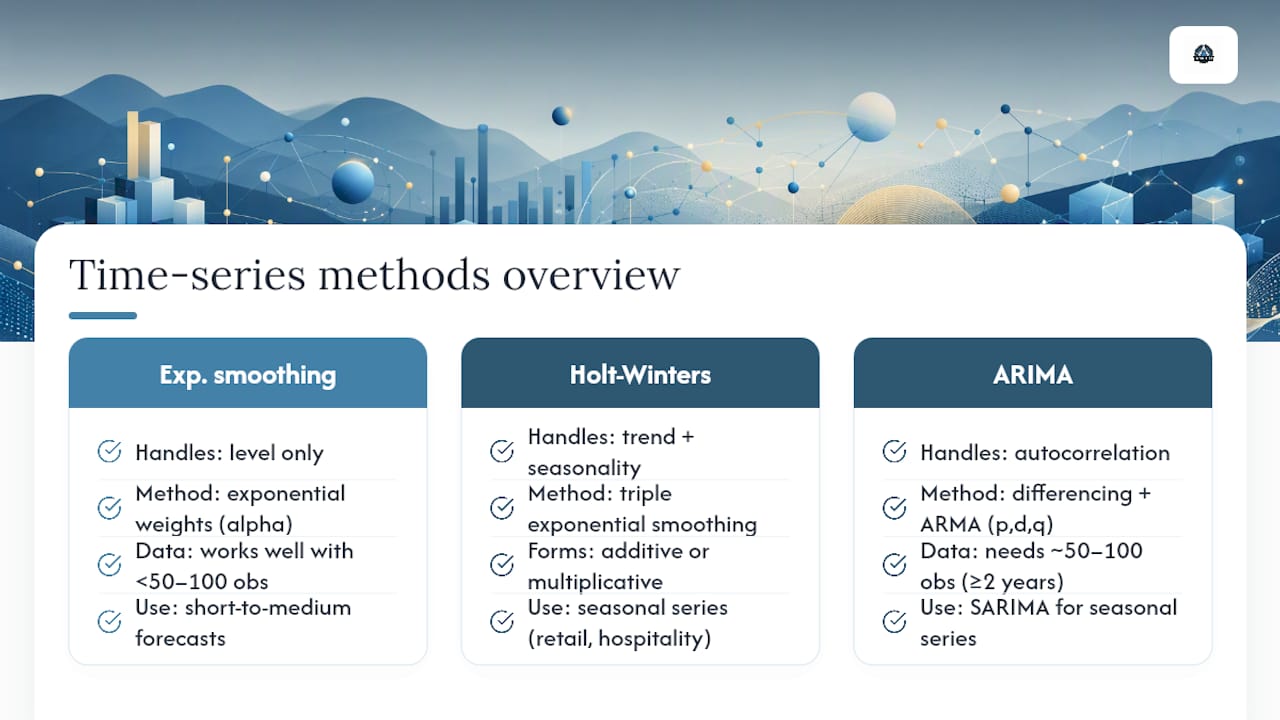
Exponential smoothing is a step up from moving averages. Instead of weighting all recent periods equally, it applies exponentially decreasing weights so that the most recent observation carries the most influence. The smoothing parameter (alpha) controls how quickly the model "forgets" older data. A high alpha makes the forecast reactive; a low alpha makes it stable. Simple exponential smoothing handles level only. When your data has a trend, you need double exponential smoothing (Holt's method). When it has both trend and seasonality, Holt-Winters (triple exponential smoothing) is the standard choice — available in both additive and multiplicative forms depending on whether seasonal swings are constant or proportional to the level.
ARIMA (AutoRegressive Integrated Moving Average) is more powerful and more demanding. It models autocorrelation in the series — the degree to which today's value depends on yesterday's — and uses differencing to handle trends and make the series stationary. SARIMA extends ARIMA to handle seasonal patterns explicitly. The tradeoff: ARIMA requires at least two years of data at the forecast frequency, a stationarity check (ADF test), and parameter selection (p, d, q) that requires statistical judgment or automated tools like auto.arima in R or statsmodels in Python.
Practical use cases: weekly sales forecasting, daily cash position modeling, and monthly revenue projections for businesses with clear seasonal patterns (retail, hospitality, subscription SaaS with annual renewal spikes). The minimum data requirement for reliable ARIMA is roughly 50–100 observations at the forecast frequency. Fewer than that, and exponential smoothing or even a moving average will often outperform it on held-out data.
Pro Tip: Before fitting any time-series model, plot your data. Trend breaks, outliers from one-time events, and missing periods will corrupt any model you build on top of them. Fix the data first.
How does regression analysis work in financial forecasting?
Regression models link a dependent financial variable (revenue, gross margin, operating expenses) to one or more independent predictor variables. They answer a different question than time-series models: not "what does the pattern in past values predict?" but "what drives this variable, and how much?"
Simple linear regression fits a straight line between one predictor and the outcome. The equation is Y = a + bX, where b is the coefficient that tells you how much Y changes for a one-unit increase in X. A retailer might regress monthly revenue on units sold; a SaaS company might regress MRR on the number of active accounts. The coefficient is directly interpretable: if b = $45, each additional unit sold adds $45 to revenue.
Multiple regression adds more predictors. A more realistic revenue model might include units sold, average selling price, marketing spend, and a seasonality dummy variable for Q4. The equation becomes Y = a + b₁X₁ + b₂X₂ + ... + bₙXₙ. This is where regression analysis in finance gets genuinely useful — and where it gets dangerous if you skip the diagnostics.
Before trusting a regression forecast, check these:
- R² and adjusted R²: how much variance in Y does the model explain? Adjusted R² penalizes for adding predictors that don't help.
- Residual analysis: plot residuals against fitted values. A pattern in the residuals means the model is missing something systematic.
- Heteroskedasticity: if residual variance grows with the fitted value, your standard errors are wrong and your confidence intervals are unreliable.
- Multicollinearity: if two predictors are highly correlated (VIF > 10 is a common threshold), their individual coefficients become unstable and hard to interpret.
- Omitted variable bias: if a variable that genuinely drives Y is left out of the model, the coefficients on included variables absorb its effect and become misleading.
The main advantage of regression over time-series is explanatory power: you can see why revenue is expected to change, not just that it will. The main risk is overfitting — a model with too many predictors relative to observations will fit historical data beautifully and forecast future data poorly.
Bottom-up vs. top-down: which framework fits your situation?
These two frameworks represent the most fundamental structural choice in financial planning. CFI's forecasting model comparison puts it plainly: bottom-up is the standard for detailed operational budgeting; top-down is the standard for strategic planning and market sizing. Most mature finance functions use both and reconcile them.
Bottom-up (driver-based) forecasting starts at the transaction level and builds up. The drivers are the operational levers: units sold, average revenue per user (ARPU), conversion rates, headcount, and cost per hire. A simple example: a SaaS company forecasts new ARR as new customers × average contract value, then adds that to existing ARR net of churn. Each driver is owned by a business unit, which makes the forecast both more accurate and more accountable.
Mini pro forma illustration: if a company projects 200 new customers at an average contract value of $12,000, new ARR = $2.4M. That $10M flows into the pro forma income statement as revenue, which then drives COGS (at the historical margin), gross profit, and operating expenses — producing a complete three-statement forecast from a single driver assumption.
Top-down forecasting starts from the market. You estimate total addressable market (TAM), apply a realistic market share assumption, and derive a revenue target. Macroeconomic indicators — GDP growth, sector-specific indices — inform the TAM estimate. This is where IMF GDP data and industry reports become direct model inputs rather than background context.
| Dimension | Bottom-up (driver-based) | Top-down |
|---|---|---|
| Best for | Operational budgeting, unit economics | Strategic sizing, market-entry, investor decks |
| Forecast horizon | Short to medium (monthly to annual) | Medium to long (annual to 5-year) |
| Data required | Granular operational data, CRM, ERP | Market data, macro indicators, industry benchmarks |
| Complexity | Moderate; requires driver ownership | Low to moderate; fewer variables |
| Output type | Detailed line-item point estimates | High-level revenue/margin ranges |
| Interpretability | High; each driver is explainable | High; assumptions are visible |
The best practice is to run both and reconcile. If your bottom-up drivers produce a revenue forecast that implies a high or unrealistic market share in year two, your top-down check will catch that before it reaches the board.
Scenario analysis and Monte Carlo: forecasting under uncertainty
Point forecasts are useful. Probabilistic forecasts are more honest. Scenario analysis and Monte Carlo simulation are the two main tools for converting a single-point assumption into a range that reflects real uncertainty.
Scenario analysis builds three or more discrete versions of the future: a base case (most likely), an upside case (favorable conditions), and a downside or stress case (adverse conditions). Each scenario gets its own set of driver assumptions. The output is a set of financial statements for each scenario, which lets leadership see the liquidity buffer required to survive the downside before it happens.
Setting realistic scenario drivers is the hard part. Revenue shocks, margin compression, and cost spikes should be grounded in historical precedent or macro data — not invented. GDP contraction rates from IMF data, sector-specific margin histories, and your own worst historical quarters are all legitimate anchors.
Monte Carlo simulation goes further. Instead of three discrete scenarios, it treats each key input (revenue growth rate, gross margin, customer churn) as a probability distribution and samples from those distributions thousands of times to generate a full distribution of possible outcomes. That kind of output is far more useful for sizing a credit facility or setting a cash reserve than a single base-case number.

The tradeoff: Monte Carlo requires you to specify input distributions, which is itself an assumption-heavy exercise. If you assume revenue growth is normally distributed when it's actually fat-tailed, your probability outputs will understate tail risk. Use it where the decision genuinely requires probabilistic thinking — capital allocation, debt covenant stress testing, M&A valuation — and keep scenario analysis for the more routine planning cycle.
When does machine learning actually improve financial forecasts?
Machine learning adds genuine value in a narrow set of conditions: you have a large, clean dataset (typically thousands of observations), the relationships between predictors and the outcome are non-linear, and you have the technical infrastructure to build, validate, and maintain the models responsibly.
Common algorithm families used in financial forecasting:
- Random forests and gradient boosting (XGBoost, LightGBM): strong for tabular data with many predictors; handle non-linearities and interactions automatically; widely used for expense forecasting and credit risk.
- LSTM (Long Short-Term Memory) networks: a type of recurrent neural network suited to sequential data; used for multi-step revenue or demand forecasting where temporal dependencies are complex.
- Prophet (Meta's open-source library): designed specifically for business time-series with strong seasonality and holiday effects; accessible to finance teams without deep ML expertise.
The governance requirements are non-negotiable. Feature engineering (deciding which variables to include and how to transform them), cross-validation on time-series splits (not random splits, which leak future data into training), model versioning, and stakeholder explainability are all prerequisites — not optional extras. Without them, an ML model is a black box that produces numbers no CFO can defend to a board.
When to skip ML entirely: sparse data (fewer than a few hundred observations), low data quality, or any situation where a regulator, auditor, or board member will ask "why did the model predict that?" and you need a clear answer. In those cases, a well-specified regression or a driver-based model will outperform ML on both accuracy and trust.
Qualitative methods: Delphi, expert panels, and market research
When the data doesn't exist or can't be trusted, structured judgment is the only tool available. Qualitative forecasting methods are not a fallback for lazy analysts — they are the appropriate choice for new product launches, market-entry decisions, post-disruption reforecasting, and any situation where structural change has broken the historical record.
The Delphi method is the most rigorous qualitative approach. University of Edinburgh's research center describes it as a structured, iterative process: a facilitator collects anonymous forecasts from a panel of experts, shares the aggregated results back to the group, and repeats the process until the panel converges on a consensus range. Anonymity prevents any single expert from dominating the discussion, and iteration allows participants to revise their estimates in light of the group's reasoning. Research published in PMC confirms that Delphi produces more reliable consensus estimates than unstructured expert discussions, particularly when the domain involves genuine uncertainty and diverse expertise.
Expert panels are less formal: a group of internal and external subject-matter experts provides structured input on market size, competitive dynamics, or technology adoption curves. The output is typically a range of estimates with documented assumptions rather than a single number.
Market research — surveys, conjoint analysis, customer interviews — generates demand-side data for new products where no sales history exists. It's the standard input for a new-product pro forma when you're building a top-down revenue estimate from scratch.
The practical integration: use qualitative inputs to set the bounds of your scenario analysis, then run quantitative models within those bounds.
How to choose the right forecasting model for your business
Model selection is a decision, not a discovery. HighRadius's forecasting taxonomy recommends matching model type to use case based on data availability and horizon — a principle that holds across every industry and company size.
Work through these questions in order:
- What decision will this forecast inform? Cash management requires daily or weekly accuracy. Strategic planning tolerates wider ranges over longer horizons. The decision defines the required precision and horizon before you touch a spreadsheet.
- What is your forecast horizon? Short-term (weekly to quarterly) favors time-series and moving averages. Medium-term (quarterly to annual) favors driver-based and regression models. Long-term (multi-year) favors top-down with scenario analysis.
- How much historical data do you have, and how clean is it? Less than 12 months of consistent data rules out most time-series methods. Structural breaks (COVID, a major product pivot) may require you to treat pre-break and post-break data separately.
- How explainable does the output need to be? A board presentation requires a model where every assumption is visible. An internal cash desk can tolerate a black-box ARIMA if it's accurate. Stakeholder explainability is a hard constraint, not a preference.
- What are your technical resources? Excel handles percent-of-sales, straight-line, moving averages, and basic regression. Statistical packages (R, Python) handle ARIMA, Holt-Winters, and ML. Dedicated FP&A platforms (Anaplan, Planful, Vena) handle driver-based models with built-in workflow and version control.
A prioritized selection order: data availability first, then horizon, then explainability requirements, then tooling. Start with the simplest model that meets your data and horizon constraints. Escalate complexity only when a more complex model produces measurably lower error on a held-out test period.
Pro Tip: Keep a simple baseline model — a moving average or straight-line growth rate — running alongside any complex model. If the complex model starts diverging significantly from the baseline without a clear business reason, that divergence is a warning sign worth investigating before it reaches a planning cycle.
Inputs, assumptions, and how to evaluate forecast accuracy
A forecast is only as good as its inputs. Before selecting a method, audit your data sources and document every assumption that feeds the model.
Common data inputs by source:
- ERP systems (SAP, Oracle, NetSuite): historical revenue, COGS, operating expenses
- POS systems: transaction-level sales data, product mix, channel splits
- CRM pipeline (Salesforce, HubSpot): weighted pipeline, conversion rates, deal velocity
- Payroll ledger: headcount, compensation, benefit costs
- Bank feeds: actual cash positions, payment timing, receivables aging
Frequency matters as much as source. A model built on monthly data cannot reliably produce weekly forecasts. Match your data frequency to your forecast frequency, and flag any gaps or imputed values in your assumption documentation.
Evaluation metrics are how you know whether a model is worth using. Three are standard:
- MAPE (Mean Absolute Percentage Error): average of absolute percentage errors across forecast periods. Formula: MAPE = (1/n) × Σ |Actual − Forecast| / Actual × 100. A MAPE of 8% means your forecast is off by 8% on average. Useful for comparing models across different scales; breaks down when actuals are near zero.
- RMSE (Root Mean Squared Error): square root of the average squared errors. Penalizes large errors more heavily than MAPE. Use RMSE when large misses are disproportionately costly.
- MAE (Mean Absolute Error): average of absolute errors without squaring. More robust to outliers than RMSE; easier to interpret in dollar terms.
Always evaluate on a holdout period — data the model never saw during training. Academic research on model evaluation confirms that horizon-specific backtesting on holdout periods is the only reliable way to compare model performance; a single aggregate metric across all horizons can mask poor performance at the specific horizon you care about.
Operationalizing forecasts: cadence, ownership, and common pitfalls
Building a model is the easy part. Getting it into a regular planning cadence that actually improves decisions is where most teams struggle. The SBA notes that forecasts don't need to be perfect to add value — but they do need to be used consistently and updated regularly.
Implementation checklist:
- Cadence: decide between a fixed forecast (annual budget with quarterly updates) and a rolling forecast (always projecting 12 or 18 months forward, updated monthly). Rolling forecasts are more responsive but require more discipline to maintain.
- Ownership: assign a data owner (who pulls and validates inputs), a model owner (who runs and updates the model), and a business owner (who reviews outputs and signs off on assumptions). Without clear ownership, models drift and go stale.
- Version control: save each forecast version with a timestamp and a change log. When actuals diverge from forecast, you need to know whether the miss was a model error, a data error, or a genuine business surprise.
- Governance: establish a sign-off process before any forecast is used in a board deck, a loan covenant calculation, or a hiring decision.
Common pitfalls:
- Treating a single model as the source of truth. Every model has blind spots. Run at least two approaches and reconcile the differences.
- Ignoring data quality. Garbage in, garbage out — a sophisticated ARIMA model built on unreconciled ledger data will produce precise nonsense.
- Failing to monitor drift. A model calibrated in 2023 may be systematically biased by 2026 if the business has changed. Quarterly recalibration is a minimum.
- Skipping backtesting. If you haven't tested the model on data it didn't see, you don't know whether it works.
Software stack by complexity: Excel and Google Sheets handle simple methods and basic regression. R and Python handle time-series, ARIMA, and ML. Dedicated FP&A platforms like Anaplan, Planful, or Vena handle driver-based models with workflow, collaboration, and audit trails built in. Match the tool to the model, not to what the team already knows.
Amcfo's recommendation: use a hybrid approach with a structured checklist
The single most important recommendation for any finance team building or improving a forecasting process: prefer a hybrid workflow that uses top-down market validation to check bottom-up driver forecasts, and automate monitoring wherever possible.
Here is the step-by-step checklist Amcfo uses with clients:
- Define the decision use. What will this forecast actually drive — a hiring plan, a credit facility, a board presentation? The answer determines required precision, horizon, and update frequency.
- Select a baseline model. Start with the simplest method that fits your data depth and horizon. Document why you chose it.
- Validate against a top-down market check. If your bottom-up drivers imply a revenue number, sanity-check it against TAM, market growth rates, and your historical win rate. A bottom-up forecast that implies implausible market share is a red flag, not a plan.
- Run scenario tests. Build at least a base, upside, and downside case. Stress-test the downside against a realistic shock (demand drop, cost spike, key customer loss).
- Monitor performance metrics and recalibrate quarterly. Track MAPE or RMSE against actuals each period. If error is trending up, investigate before the next planning cycle.
The rationale for this hybrid approach: bottom-up models capture operational reality but can drift from market context; top-down models capture macro trends but miss operational constraints. Running both and reconciling the gap produces a forecast that is both defensible to a board and actionable for a business unit. It also creates an audit trail — every assumption is documented, every model version is saved, and every variance has an explanation.
Pro Tip: Keep at least one simple, explainable baseline model alongside any complex model. When a sophisticated model produces a surprising output, the baseline tells you immediately whether the surprise is real or a model artifact. That single habit saves hours of troubleshooting and preserves stakeholder trust.
What fractional CFOs actually fix in broken forecasting processes
The most common mistake finance teams make is not choosing the wrong model — it's choosing no model at all and calling a spreadsheet with last year's numbers a forecast. The second most common mistake is building a model that no one updates, validates, or owns after the initial build.
In a typical Amcfo engagement, a client arrives with one of three problems: a forecast that hasn't been backtested against actuals in over a year, a model built on unreconciled data from three different systems that don't agree, or a planning process where the CFO and the business unit leads are working from different versions of the same spreadsheet. None of these are model-selection problems. They are governance and data problems that make any model unreliable regardless of its sophistication.
The fix is usually less glamorous than the client expects: reconcile the data sources, establish a single version of truth, assign ownership, and set a quarterly recalibration cadence. Once that foundation is in place, moving a client from a static annual budget to a rolling 12-month driver-based forecast typically takes one to two quarters. The model itself is the easy part. Getting the organization to trust it and act on it is the work.
Fractional CFOs add value at exactly the intersection where model sophistication and organizational readiness meet. They can build a financial forecasting process that matches the company's actual data maturity, connect the forecast to the decisions that matter, and train the internal team to maintain it without ongoing external support.
Amcfo's forecasting and modeling services
Amcfo's fractional CFO services are built around exactly the hybrid framework this article describes. For businesses that need a forecast but don't have the internal bandwidth to build and maintain one, Amcfo handles the full process: selecting the right model family for your data and decision horizon, building the driver-based or time-series model, integrating it with your QuickBooks or ERP data, and setting up the quarterly recalibration cadence that keeps it accurate.

Service formats include a one-time model build (project-based, with documentation and handoff training), a monthly retainer for ongoing monitoring, variance analysis, and updates, and a forecasting health check for teams that already have a model but aren't sure whether to trust it. For businesses that need cleaner data before any model will work, Amcfo's accounting and bookkeeping services provide the reconciled, consistent financial records that every reliable forecast depends on. Schedule a diagnostics call to find out which model type fits your business and what it would take to get your forecasting process running reliably.
Sources
- Forecasting Model Comparison: When You Should Use Each | CFI
- Financial Forecasting Models and Methods | IBM
- 7 Financial Forecasting Methods to Predict Business Performance
- Gross domestic product (GDP) — IMF
This article is general information, not a substitute for advice from a qualified financial advisor. Consult a qualified financial professional about your own circumstances before acting on anything here.